Stefan problem
In mathematics and its applications, particularly to phase transitions in matter, a Stefan problem (also Stefan task) is a particular kind of boundary value problem for a partial differential equation (PDE), adapted to the case in which a phase boundary can move with time. The classical Stefan problem aims to describe the temperature distribution in a homogeneous medium undergoing a phase change, for example ice passing to water: this is accomplished by solving the heat equation imposing the initial temperature distribution on the whole medium, and a particular boundary condition, the Stefan condition, on the evolving boundary between its two phases. Note that this evolving boundary is an unknown (hyper-)surface: hence, Stefan problems are examples of free boundary problems.
Contents |
Historical note
The problem is named after Jožef Stefan, the Slovene physicist who introduced the general class of such problems around 1890, in relation to problems of ice formation. This question had been considered earlier, in 1831, by Lamé and Clapeyron.
Premises to the mathematical description
From a mathematical point of view, the phases are merely regions in which the coefficients of the underlying PDE are continuous and differentiable up to the order of the PDE. In physical problems such coefficients represent properties of the medium for each phase. The moving boundaries (or interfaces) are infinitesimally thin surfaces that separate adjacent phases; therefore, the coefficients of the underlying PDE and its derivatives may suffer discontinuities across interfaces.
The underlying PDE is not valid at phase change interfaces; therefore, an additional condition—the Stefan condition—is needed to obtain closure. The Stefan condition expresses the local velocity of a moving boundary, as a function of quantities evaluated at both sides of the phase boundary, and is usually derived from a physical constraint. In problems of heat transfer with phase change, for instance, the physical constraint is that of conservation of energy, and the local velocity of the interface depends on the heat flux discontinuity at the interface.
Mathematical formulation
The one-dimensional one-phase Stefan problem
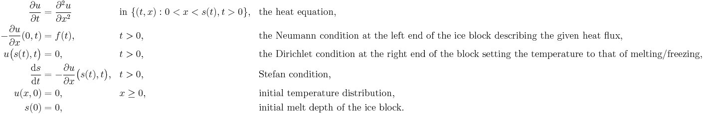
Consider an semi-infinite one-dimensional block of ice initially at melting temperature  ≡
≡ for
for  ∈ [0,+∞[. The ice is heated from the left with heat flux
  . The flux causes the block to melt down leaving an interval
 ![[0,s(t)]](/2012-wikipedia_en_all_nopic_01_2012/I/2a4da84c0f3b35c8135389d847e04a4c.png) occupied by water. The melt depth of the ice block, denoted by
occupied by water. The melt depth of the ice block, denoted by  , is an unknown function of time; the solution of the Stefan problem consists of finding and
  such that
The Stefan problem also has a rich inverse theory, where one is given the curve and the problem is to find or  .
.
Applications
The solution of the Cahn–Hilliard equation for a binary mixture demonstrated to coincide well with the solution of a Stefan problem.[1]
See also
- Free boundary problem
- Moving boundary problem
- Olga Arsenievna Oleinik
- Shoshana Kamin
- Stefan's equation
Notes
- ^ F. J. Vermolen, M.G. Gharasoo, P. L. J. Zitha, J. Bruining. (2009). Numerical Solutions of Some Diffuse Interface Problems: The Cahn-Hilliard Equation and the Model of Thomas and Windle. IntJMultCompEng,7(6):523–543.
References
- Vuik, C. (1993), "Some historical notes about the Stefan problem", Nieuw Archief voor Wiskunde, 4e serie 11: 157–167, MR1239620, Zbl 0801.35002. An interesting historical paper on the early days of the theory: a preprint version (in PDF format) is available here.
Bibliography
- Cannon, John Rozier (1984), The One-Dimensional Heat Equation, Encyclopedia of Mathematics and Its Applications, 23 (1st ed.), Reading–Menlo Park–London–Don Mills–Sidney–Tokyo/ Cambridge–New York–New Rochelle–Melbourne–Sidney: Addison-Wesley Publishing Company/Cambridge University Press, pp. XXV+483, ISBN 9780521302432, MR0747979, Zbl 0567.35001, http://books.google.com/?id=XWSnBZxbz2oC&printsec=frontcover#v=onepage&q=. Contains an extensive bibliography of 460 items on the Stefan and other free boundary problems, updated to 1982.
- Kirsch, Andreas (1996), Introduction to the Mathematical Theory of Inverse Problems, Applied Mathematical Sciences series, 120, Berlin–Heidelberg–New York: Springer Verlag, pp. x+282, ISBN 0-387-94530-X, MR1479408, Zbl 0865.35004, http://books.google.com/books?id=llNUaSKHj3gC&printsec=frontcover#v=onepage&q&f=true
- Meirmanov, Anvarbek M. (1992), The Stefan Problem, De Gruyter Expositions in Mathematics, 3, Berlin-New York: Walter de Gruyter, pp. x+245, ISBN 3-11-011479-8, MR1154310, Zbl 0751.35052, http://books.google.com/?id=ae1VlQjOtJQC&printsec=frontcover#v=onepage&q=.
- Oleinink, O.A. (1960), "A method of solution of the general Stefan problem" (in Russian), Doklady Akademii Nauk SSSR 135: 1050–1057, MR0125341, Zbl 0131.09202. In this paper, for the first time and independently of S.L. Kamenomostskaya, the author proves the existence of a generalized solution for the three-dimensional Stefan problem.
- Kamenomostskaya, S.L. (1961), "On Stefan's problem" (in Russian), Matematicheskii Sbornik 53(95) (4): 489–514, MR0141895, Zbl 0102.09301, http://mi.mathnet.ru/eng/msb/v95/i4/p489. In this paper, for the first time and independently of Olga Oleinik, the author proves the existence and uniqueness of a generalized solution for the three-dimensional Stefan problem.
- Rubinstein, L.I. (1994), The Stefan Problem, Translations of Mathematical Monographs, 27, Providence, R.I.: American Mathematical Society, pp. viii+419, ISBN 0-8218-1577-6, MR0351348, Zbl 0219.35043, http://books.google.com/?id=lDnLwUyiGAwC&printsec=frontcover#v=onepage&q=. A comprehensive reference updated up to 1962–1963, with a bibliography of 201 items.
- Tarzia, Domingo Alberto (Julio 2000), "A Bibliography on Moving-Free Boundary Problems for the Heat-Diffusion Equation. The Stefan and Related Problems", MAT, Series A: Conferencias, seminarios y trabajos de matemática. 2: 1–297, ISSN 1515-4904, MR1802028, Zbl 0963.35207, http://web.austral.edu.ar/cienciasEmpresariales-investigacion-mat-A-02.asp. The impressive personal bibliography of the author on moving and free boundary problems (M–FBP) for the heat-diffusion equation (H–-DE), containing about 5900 references to works appeared on approximately 884 different kinds of publications. Its declared objective is trying to give a comprehensive account of the western existing mathematical–physical–engineering literature on this research field. Almost all the material on the subject, published after the historical and first paper of Lamé–Clapeyron (1831), has been collected. Sources include scientific journals, symposium or conference proceedings, technical reports and books.
External links
- Vasil'ev, F. P. (2001), "Stefan condition", in Hazewinkel, Michiel, Encyclopedia of Mathematics, Springer, ISBN 978-1556080104, http://www.encyclopediaofmath.org/index.php?title=S/s087590
- Vasil'ev, F. P. (2001), "Stefan problem", in Hazewinkel, Michiel, Encyclopedia of Mathematics, Springer, ISBN 978-1556080104, http://www.encyclopediaofmath.org/index.php?title=S/s087600
- Vasil'ev, F. P. (2001), "Stefan problem, inverse", in Hazewinkel, Michiel, Encyclopedia of Mathematics, Springer, ISBN 978-1556080104, http://www.encyclopediaofmath.org/index.php?title=S/s087610